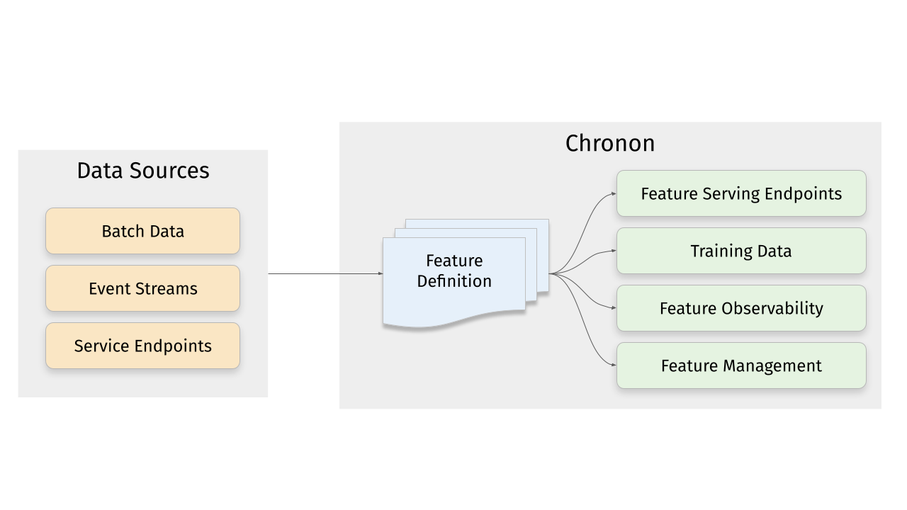
Chronon is a platform that abstracts away the complexity of data computation and serving for AI/ML applications. Users define features as transformation of raw data, then Chronon can perform batch and streaming computation, scalable backfills, low-latency serving, guaranteed correctness and consistency, as well as a host of observability and monitoring tools.

It allows you to utilize all of the data within your organization, from batch tables, event streams or services to power your AI/ML projects, without needing to worry about all the complex orchestration that this would usually entail.

More information about Chronon can be found at chronon.ai.

Chronon offers an API for realtime fetching which returns up-to-date values for your features. It supports:

• Managed pipelines for batch and realtime feature computation and updates to the serving backend
• Low latency serving of computed features
• Scalable for high fanout feature sets

ML practitioners often need historical views of feature values for model training and evaluation. Chronon's backfills are:

• Scalable for large time windows
• Resilient to highly skewed data
• Point-in-time accurate such that consistency with online serving is guaranteed

Chronon offers visibility into:

• Data freshness - ensure that online values are being updated in realtime
• Online/Offline consistency - ensure that backfill data for model training and evaluation is consistent with what is being observed in online serving

Chronon supports a range of aggregation types. For a full list see the documentation here.

These aggregations can all be configured to be computed over arbitrary window sizes.

This section walks you through the steps to create a training dataset with Chronon, using a fabricated underlying raw dataset.

Includes:

• Example implementation of the main API components for defining features - GroupBy and Join.
• The workflow for authoring these entities.
• The workflow for backfilling training data.
• The workflows for uploading and serving this data.
• The workflow for measuring consistency between backfilled training data and online inference data.

Does not include:

• A deep dive on the various concepts and terminologies in Chronon. For that, please see the Introductory documentation.
• Running streaming jobs.

• Docker

To get started with the Chronon, all you need to do is download the docker-compose.yml file and run it locally:

curl -o docker-compose.yml https://chronon.ai/docker-compose.yml
docker-compose up

Once you see some data printed with a only showing top 20 rows notice, you're ready to proceed with the tutorial.

In this example, let's assume that we're a large online retailer, and we've detected a fraud vector based on users making purchases and later returning items. We want to train a model that will be called when the checkout flow commences and predicts whether this transaction is likely to result in a fraudulent return.

Fabricated raw data is included in the data directory. It includes four tables:

1. Users - includes basic information about users such as account created date; modeled as a batch data source that updates daily
2. Purchases - a log of all purchases by users; modeled as a log table with a streaming (i.e. Kafka) event-bus counterpart
3. Returns - a log of all returns made by users; modeled as a log table with a streaming (i.e. Kafka) event-bus counterpart
4. Checkouts - a log of all checkout events; this is the event that drives our model predictions

In a new terminal window, run:

docker-compose exec main bash

This will open a shell within the chronon docker container.

Now that the setup steps are complete, we can start creating and testing various Chronon objects to define transformation and aggregations, and generate data.

Let's start with three feature sets, built on top of our raw input sources.

Note: These python definitions are already in your chronon image. There's nothing for you to run until Step 3 - Backfilling Data when you'll run computation for these definitions.

Feature set 1: Purchases data features

We can aggregate the purchases log data to the user level, to give us a view into this user's previous activity on our platform. Specifically, we can compute SUMs COUNTs and AVERAGEs of their previous purchase amounts over various windows.

Because this feature is built upon a source that includes both a table and a topic, its features can be computed in both batch and streaming.

source = Source(
    events=EventSource(
        table="data.purchases", # This points to the log table with historical purchase events
        topic=None, # Streaming is not currently part of quickstart, but this would be where you define the topic for realtime events
        query=Query(
            selects=select("user_id","purchase_price"), # Select the fields we care about
            time_column="ts") # The event time
    ))

window_sizes = [Window(length=day, timeUnit=TimeUnit.DAYS) for day in [3, 14, 30]] # Define some window sizes to use below

v1 = GroupBy(
    sources=[source],
    keys=["user_id"], # We are aggregating by user
    aggregations=[Aggregation(
            input_column="purchase_price",
            operation=Operation.SUM,
            windows=window_sizes
        ), # The sum of purchases prices in various windows
        Aggregation(
            input_column="purchase_price",
            operation=Operation.COUNT,
            windows=window_sizes
        ), # The count of purchases in various windows
        Aggregation(
            input_column="purchase_price",
            operation=Operation.AVERAGE,
            windows=window_sizes
        ) # The average purchases by user in various windows
    ],
)

See the whole code file here: purchases GroupBy. This is also in your docker image. We'll be running computation for it and the other GroupBys in Step 3 - Backfilling Data.

Feature set 2: Returns data features

We perform a similar set of aggregations on returns data in the returns GroupBy. The code is not included here because it looks similar to the above example.

Feature set 3: User data features

Turning User data into features is a littler simpler, primarily because there are no aggregations to include. In this case, the primary key of the source data is the same as the primary key of the feature, so we're simply extracting column values rather than performing aggregations over rows:

source = Source(
    entities=EntitySource(
        snapshotTable="data.users", # This points to a table that contains daily snapshots of the entire product catalog
        query=Query(
            selects=select("user_id","account_created_ds","email_verified"), # Select the fields we care about
        )
    ))

v1 = GroupBy(
    sources=[source],
    keys=["user_id"], # Primary key is the same as the primary key for the source table
    aggregations=None # In this case, there are no aggregations or windows to define
) 

Taken from the users GroupBy.

Next, we need the features that we previously defined backfilled in a single table for model training. This can be achieved using the Join API.

For our use case, it's very important that features are computed as of the correct timestamp. Because our model runs when the checkout flow begins, we'll want to be sure to use the corresponding timestamp in our backfill, such that features values for model training logically match what the model will see in online inference.

Join is the API that drives feature backfills for training data. It primarilly performs the following functions:

1. Combines many features together into a wide view (hence the name Join).
2. Defines the primary keys and timestamps for which feature backfills should be performed. Chronon can then guarantee that feature values are correct as of this timestamp.
3. Performs scalable backfills.

Here is what our join looks like:

source = Source(
    events=EventSource(
        table="data.checkouts", 
        query=Query(
            selects=select("user_id"), # The primary key used to join various GroupBys together
            time_column="ts",
            ) # The event time used to compute feature values as-of
    ))

v1 = Join(  
    left=source,
    right_parts=[JoinPart(group_by=group_by) for group_by in [purchases_v1, refunds_v1, users]] # Include the three GroupBys
)

Taken from the training_set Join.

The left side of the join is what defines the timestamps and primary keys for the backfill (notice that it is built on top of the checkout event, as dictated by our use case).

Note that this Join combines the above three GroupBys into one data definition. In the next step, we'll run the command to execute computation for this whole pipeline.

Once the join is defined, we compile it using this command:

compile.py --conf=joins/quickstart/training_set.py

This converts it into a thrift definition that we can submit to spark with the following command:

run.py --conf production/joins/quickstart/training_set.v1

The output of the backfill would contain the user_id and ts columns from the left source, as well as the 11 feature columns from the three GroupBys that we created.

Feature values would be computed for each user_id and ts on the left side, with guaranteed temporal accuracy. So, for example, if one of the rows on the left was for user_id = 123 and ts = 2023-10-01 10:11:23.195, then the purchase_price_avg_30d feature would be computed for that user with a precise 30 day window ending on that timestamp.

You can now query the backfilled data using the spark sql shell:

spark-sql

And then:

spark-sql> SELECT user_id, quickstart_returns_v1_refund_amt_sum_30d, quickstart_purchases_v1_purchase_price_sum_14d, quickstart_users_v1_email_verified from default.quickstart_training_set_v1 limit 100;

Note that this only selects a few columns. You can also run a select * from default.quickstart_training_set_v1 limit 100 to see all columns, however, note that the table is quite wide and the results might not be very readable on your screen.

To exit the sql shell you can run:

spark-sql> quit;

Now that we've created a join and backfilled data, the next step would be to train a model. That is not part of this tutorial, but assuming it was complete, the next step after that would be to productionize the model online. To do this, we need to be able to fetch feature vectors for model inference. That's what this next section covers.

In order to serve online flows, we first need the data uploaded to the online KV store. This is different than the backfill that we ran in the previous step in two ways:

1. The data is not a historic backfill, but rather the most up-to-date feature values for each primary key.
2. The datastore is a transactional KV store suitable for point lookups. We use MongoDB in the docker image, however you are free to integrate with a database of your choice.

Upload the purchases GroupBy:

run.py --mode upload --conf production/group_bys/quickstart/purchases.v1 --ds  2023-12-01

spark-submit --class ai.chronon.quickstart.online.Spark2MongoLoader --master local[*] /srv/onlineImpl/target/scala-2.12/mongo-online-impl-assembly-0.1.0-SNAPSHOT.jar default.quickstart_purchases_v1_upload mongodb://admin:admin@mongodb:27017/?authSource=admin

Upload the returns GroupBy:

run.py --mode upload --conf production/group_bys/quickstart/returns.v1 --ds  2023-12-01

spark-submit --class ai.chronon.quickstart.online.Spark2MongoLoader --master local[*] /srv/onlineImpl/target/scala-2.12/mongo-online-impl-assembly-0.1.0-SNAPSHOT.jar default.quickstart_returns_v1_upload mongodb://admin:admin@mongodb:27017/?authSource=admin

If we want to use the FetchJoin api rather than FetchGroupby, then we also need to upload the join metadata:

run.py --mode metadata-upload --conf production/joins/quickstart/training_set.v2

This makes it so that the online fetcher knows how to take a request for this join and break it up into individual GroupBy requests, returning the unified vector, similar to how the Join backfill produces the wide view table with all features.

With the above entities defined, you can now easily fetch feature vectors with a simple API call.

Fetching a join:

run.py --mode fetch --type join --name quickstart/training_set.v2 -k '{"user_id":"5"}'

You can also fetch a single GroupBy (this would not require the Join metadata upload step performed earlier):

run.py --mode fetch --type group-by --name quickstart/purchases.v1 -k '{"user_id":"5"}'

For production, the Java client is usually embedded directly into services.

Map<String, String> keyMap = new HashMap<>();
keyMap.put("user_id", "123");
Fetcher.fetch_join(new Request("quickstart/training_set_v1", keyMap))

sample response

> '{"purchase_price_avg_3d":14.3241, "purchase_price_avg_14d":11.89352, ...}'

Note: This java code is not runnable in the docker env, it is just an illustrative example.

As discussed in the introductory sections of this README, one of Chronon's core guarantees is online/offline consistency. This means that the data that you use to train your model (offline) matches the data that the model sees for production inference (online).

A key element of this is temporal accuracy. This can be phrased as: when backfilling features, the value that is produced for any given timestamp provided by the left side of the join should be the same as what would have been returned online if that feature was fetched at that particular timestamp.

Chronon not only guarantees this temporal accuracy, but also offers a way to measure it.

The measurement pipeline starts with the logs of the online fetch requests. These logs include the primary keys and timestamp of the request, along with the fetched feature values. Chronon then passes the keys and timestamps to a Join backfill as the left side, asking the compute engine to backfill the feature values. It then compares the backfilled values to actual fetched values to measure consistency.

Step 1: log fetches

First, make sure you've ran a few fetch requests. Run:

run.py --mode fetch --type join --name quickstart/training_set.v2 -k '{"user_id":"5"}'

A few times to generate some fetches.

With that complete, you can run this to create a usable log table (these commands produce a logging hive table with the correct schema):

spark-submit --class ai.chronon.quickstart.online.MongoLoggingDumper --master local[*] /srv/onlineImpl/target/scala-2.12/mongo-online-impl-assembly-0.1.0-SNAPSHOT.jar default.chronon_log_table mongodb://admin:admin@mongodb:27017/?authSource=admin
compile.py --conf group_bys/quickstart/schema.py
run.py --mode backfill --conf production/group_bys/quickstart/schema.v1
run.py --mode log-flattener --conf production/joins/quickstart/training_set.v2 --log-table default.chronon_log_table --schema-table default.quickstart_schema_v1

This creates a default.quickstart_training_set_v2_logged table that contains the results of each of the fetch requests that you previously made, along with the timestamp at which you made them and the user that you requested.

Note: Once you run the above command, it will create and "close" the log partitions, meaning that if you make additional fetches on the same day (UTC time) it will not append. If you want to go back and generate more requests for online/offline consistency, you can drop the table (run DROP TABLE default.quickstart_training_set_v2_logged in a spark-sql shell) before rerunning the above command.

Now you can compute consistency metrics with this command:

run.py --mode consistency-metrics-compute --conf production/joins/quickstart/training_set.v2

This job takes will take the primary key(s) and timestamps from the log table (default.quickstart_training_set_v2_logged in this case), and uses those to create and run a join backfill. It then compares the backfilled results to the actual logged values that were fetched online

It produces two output tables:

1. default.quickstart_training_set_v2_consistency: A human readable table that you can query to see the results of the consistency checks.
   1. You can enter a sql shell by running spark-sql from your docker bash sesion, then query the table.
   2. Note that it has many columns (multiple metrics per feature), so you might want to run a DESC default.quickstart_training_set_v2_consistency first, then select a few columns that you care about to query.
2. default.quickstart_training_set_v2_consistency_upload: A list of KV bytes that is uploaded to the online KV store, that can be used to power online data quality monitoring flows. Not meant to be human readable.

Using chronon for your feature engineering work simplifies and improves your ML Workflow in a number of ways:

1. You can define features in one place, and use those definitions both for training data backfills and for online serving.
2. Backfills are automatically point-in-time correct, which avoids label leakage and inconsistencies between training data and online inference.
3. Orchestration for batch and streaming pipelines to keep features up to date is made simple.
4. Chronon exposes easy endpoints for feature fetching.
5. Consistency is guaranteed and measurable.

For a more detailed view into the benefits of using Chronon, see Benefits of Chronon documentation.

Chronon offers the most value to AI/ML practitioners who are trying to build "online" models that are serving requests in real-time as opposed to batch workflows.

Without Chronon, engineers working on these projects need to figure out how to get data to their models for training/eval as well as production inference. As the complexity of data going into these models increases (multiple sources, complex transformation such as windowed aggregations, etc), so does the infrastructure challenge of supporting this data plumbing.

Generally, we observed ML practitioners taking one of two approaches:

With this approach, users start with the data that is available in the online serving environment from which the model inference will run. Log relevant features to the data warehouse. Once enough data has accumulated, train the model on the logs, and serve with the same data.

Pros:

• Features used to train the model are guaranteed to be available at serving time
• The model can access service call features
• The model can access data from the the request context

Cons:

• It might take a long to accumulate enough data to train the model
• Performing windowed aggregations is not always possible (running large range queries against production databases doesn't scale, same for event streams)
• Cannot utilize the wealth of data already in the data warehouse
• Maintaining data transformation logic in the application layer is messy

With this approach, users train the model with data from the data warehouse, then figure out ways to replicate those features in the online environment.

Pros:

• You can use a broad set of data for training
• The data warehouse is well suited for large aggregations and other computationally intensive transformation

Cons:

• Often very error prone, resulting in inconsistent data between training and serving
• Requires maintaining a lot of complicated infrastructure to even get started with this approach,
• Serving features with realtime updates gets even more complicated, especially with large windowed aggregations
• Unlikely to scale well to many models

The Chronon approach

With Chronon you can use any data available in your organization, including everything in the data warehouse, any streaming source, service calls, etc, with guaranteed consistency between online and offline environments. It abstracts away the infrastructure complexity of orchestrating and maintining this data plumbing, so that users can simply define features in a simple API, and trust Chronon to handle the rest.

We welcome contributions to the Chronon project! Please read CONTRIBUTING for details.

Use the GitHub issue tracker for reporting bugs or feature requests. Join our community Discord channel for discussions, tips, and support.