CoNuS stands for "Concurrent Numerical Simulations", but the name also refers to conus sp, a genus of predatory sea snails (hence the CoNuS logo). CoNuS is a generic library for numerical stepwise modelling, and it is written in Scala. CoNuS is part of the Carbonate Shells numerical toolset, and it is currently experimental software, with active testing and coding in progress within Cédric John's research group at Imperial College London. This means that code written using CoNuS is susceptible to break in future releases as the API is not fully stable yet.
The latest version of the library is 0.2.3, running on Scala versions 2.12 and 2.13
Quick setup guide
CoNuS with SBT
CoNuS within a Jupyter Notebook
Introduction to CoNuS
The CoNuS modelling philosophy
CoNuS execution model and advantages of Scala
A step by step example
Defining a very simple model
Running your model, querying and saving results
Running multiple version of your model in parrallel
For SBT, add these lines to your SBT project definition:
resolvers += "jitpack" at "https://jitpack.io"

libraryDependencies  ++= Seq(
  // Last  release
  "org.carbonateresearch" %% "conus" % "0.2.3"
)
To access the simulator, simply create an interface to the BasicSimulator:
val sim = new BasicSimulatorThe preferred and easiest way to work with forward models using CoNuS is via notebooks. We tested CoNuS with Almond v.0.9.1. To use CoNuS within a Jupyter Notebook with the Almond kernel, first add the following resolver:
interp.repositories() ++= Seq(coursierapi.MavenRepository.of(
"https://jitpack.io"
))
Then import the CoNuS library:
import $ivy. `org.carbonateresearch::conus:0.2.3`All of the basic classes you need to work with stepped models can be imported with this wildcard import:
import org.carbonateresearch.conus._Finally, you need to create an interface to the simulator, which is the object you will use to run your code. For the Almond kernel, create an AlmondSimulator this way:
val sim = new AlmondSimulatorThis will add nice graphical output to your cells, and will ensure that CoNuS integrates well with the Jupyter notebook.
Stepwise simulation can be defined as the art of modeling a system and its changing states by dividing the modelling space into discrete 'steps'. There is often (but not always) an implicit notion of time associated with the steps, i.e. each step represents an increment in time to either later (forward models) or earlier (inverse models) time.
Stepwise simulation is a very general modelling approach that can be applied to any natural or manmade systems, such as for instance weather patterns, ocean circulation, population dynamic, financial markets, disease propagation, systems engineering, electrical grid supply and demand, to name just a fiew.
Stepwise simulation packages can be divided into two broad categories: professional packages and user code. Professional packages come with all the belts and whistles, they usually run on optimised code to maximize CPU/GPU efficiency with the most appropriate algorithm, and they typically have a nice GUI. However, professional code have their limitations too. They can be expensive, and as a user you have no control on the mathematical model used in your calculator. Also, only certain specific applications are possible with a given professional system: for instance, a stepwise simulator dedicated to model disease conrol will not be able to handle applications to weather patterns. So if a given dedicated code does not exist for your application, or if you want to slightly modify the modelling approach in your systen, chances are you won't be able to do it.
At the opposite end of this approach is pure user code: you can choose the programming language of your choice (typically C/C++, MATLAB, Python...) and implement the entire system in this language. This means you will have complete control on the mathematical model applied in your simulator, but you will also be respondible for implementing the simulator, i.e. design a grid system for your simulator, design an event loop that will run through the steps in your model one by one and store the state of your system at each simulation step, and of course, design the testing strategy that will allow you to assess how well your model has performed. In my experience as a researcher, this is very prone to error, often inefficient due to language/platform choice, and of course, it means reinventing the wheel for each new problem to be solve with a stepwise modelling approach.
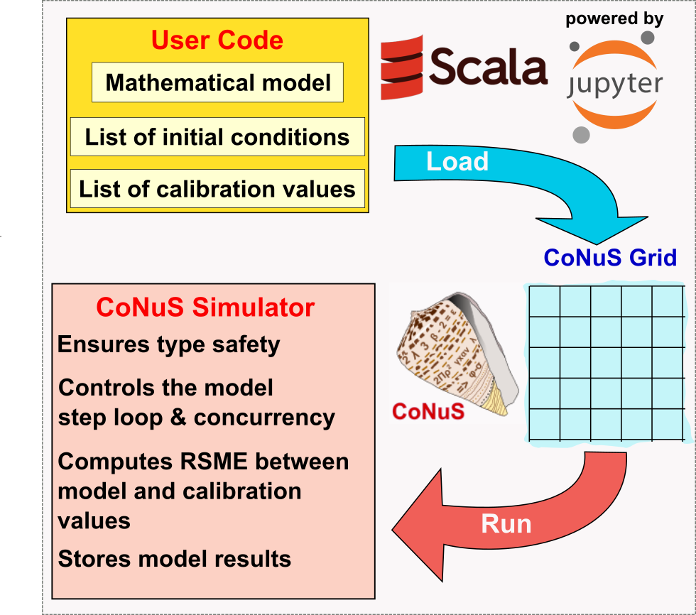 Figure 1: Architecture of CoNuS. User defined code include a mathematical model built by writing 'step functions' in Scala, as well as a list of initial conditions (the state of the model before the simulation starts) and an optional list of test for the model results against known values.
CoNuS offers an alternative model for running stepwise models (Figure 1), including the convenience of doing this into a Jupyter Notebook with the Scala Almond.sh kernel installed. In CoNuS, the user if only responsible for writing (in Scala) the mathematical model used by the simulator (using stepFunctions, more about this later) as well as providing the dimension of the model grid, inital conditions (the inital state of the model), the number of steps to run the model, as well as any model calibration code (to test how well the model performs). In other words, the user only supplies code that is directly relevant to the modelling problem.
The CoNuS library takes care of running the model for the user (Figure 1). CoNuS will load user code onto an internal representation of a grid (1D, 2D or 3D). Under the hood, we use Breeze's matrix or vector to represent the grid, as this is an efficient linear algebra library in Scala build on top of BLAS. However, this is transparent to the user and might change in the future. The CoNuS Simulator then centralises the running, evaluating and interaction with the user-created model. This ensures low overload for the library user, and the use of efficient and type-safe code.
A core concept behind the design of CoNuS is concurency and the ability to run multiple models at once (Figure 2). Scala is therefore a language of choice, as CoNuS leverages on the functional approach in Scala to write step functions for the simulator, and to use the flexibility of the Scala syntax to develope a DSL (domaine specific language) for numerical modelling. Scala is also an excellent choice for concurrent work, thanks to the availability of native support for concurrency and the Akka Actor library.
CoNuS offers the ability to define several possible initial model condition values when declaring a model variable (see Figure 2). These different initial values are then associated using combinatorial rules to create a list of all possible initial model conditions (Figure 2). We refer to this as the 'Model Calculation Space'.
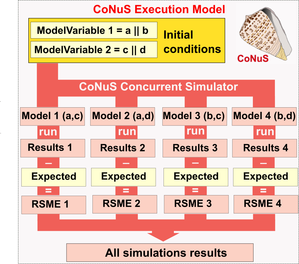 Figure 2: The CoNuS execution model. Multiple simulations can be created if a list of possible initial conditions is supplied, and a model calculation space containing all possible combinatorial models (in this case 4) is calculated by CoNuS. Execution of the model run is performed in parrallel to speed up calculation.
In Figure 2, a very simple example is provided. Two model variables each have two possible distinct initial values (a or b for model 1, c or d for model 2). With this user input, CoNuS will automatically create a model calculation space containing 4 different models that represent the possible combination of these initial conditions (Figure 2). The simulator will then run each model independently in parrallel, test the model output against the expected results (if they are provided) and calculate a root mean squared error (RSME) for each model, before storing all of the models into the simulator results for further querying by the user. This is done behind the scene using the Akka Typed framework. The ability to run multiple models in parrallel, and then assess the results of each one of them against a supplied 'truth' is one of the strenght of CoNuS.
Here we will build a very simple model. In fact, this model is not just simple, it is simplistic! But it will help you understand the coding philosophy behind CoNuS. We will assume that you are using CoNuS from a Jupyter Notebook with Almond.. This is the easiest way to interact with CoNuS and we recommend using it. Of course, you can also use CoNuS in your IDE of choice: the library can be used to build applications, for instance, a highly optimised simulator for your favorite application domaine.
The simulation we will build will try to predict rat population in a field. This is a very small simulation but it serves as an illustration of what you could do with more complex problems.
Make sure you have followed the instructions for importing the CoNuS dependencies in Almond, all the way to the line that imports the most commonly needed classes into your notebook, and the creation of your simulator (which we have named 'sim' for convenience in our code). The first step is to reason about our modelling problem.
We will simulate a wheat field where the rats live: this will be represented by a 2D CoNuS grid. The grid has a dimension of 3x3 cells, and each grid cell is meant to represent 100x100 meters of a field. We initialize the model with values ranging from 2.0 to 6.0. These represent the population of rats living in each 100 sq meter of the field. We will run the simulation for 10 time step, each time step represents one generation of rats. We assume a perfect parity between male and female rat, and we also assume that each couple will have 10 babies per generation. In addition, we will simulate a death rate between 0 to 0.9 (0 to 90% of the population), assigned randomly at each timestep and independently for each square. A major simplification is that each cell (square in the field) has its own rat population, there is no movement of rats in between the different grid cells.
So the first thing is to decide what will be calculated: the rat population and the death rate. Both of these will vary throughout the steps of the model. In other words, they represent the state of the model and need to be represented as model variables.Enter the following in a cell of your notebook and press shift+return:
// In CoNuS, values that will be calculated are known as model variables. Let's set a few:
val nbRats:ModelVariable[Int] = ModelVariable("Number of Rats",2,"Individuals") //Notice this is an Int
val deathRate:ModelVariable[Double] = ModelVariable("Death rate",0.0,"%") //This is a double. CoNuS is type safe.

// Let's initialise a variabe that sets the number of steps in our model:
val numberOfSteps = 10

// And let's create a function that, given a rat population and a deathRate, calculates a new population

def survivingRats(initialPopulation:Int, deathRate:Double): Int = {
    initialPopulation-math.floor(initialPopulation.toDouble*deathRate).toInt
}
Of course, Scala comments ('//') are optional and do not need to be typed. Because this is such as simple model, we are now ready to write the CoNuS code for the model:
// We will call our model 'ratPopulation'
val ratPopulation = new SteppedModel(numberOfSteps,"Simplified rat population dynamics") //Notice that we give the number of steps, and a long name for the model as a string
    .setGrid(3,3) // This sets the 2D grid, or a 3x3 = 9 cells grid.
    .defineMathematicalModel( // In this super simple model we do only two things at each step
      deathRate =>> {(s:Step) => scala.util.Random.nextDouble()*0.9}, // calculate a death rate
      nbRats =>> {(s:Step) => {survivingRats(nbRats(s-1)+(nbRats(s-1)/2*10),deathRate(s))}} // calcuate the nb rats
    )
    .defineInitialModelConditions( // Now we need to determine the inital size of the population at each model grid
      PerCell(nbRats,List(
        (List(2),Seq(0,0)), // This sets 1 unique value of 2 for cell 0,0. The other lines do the same, with different values for different grid coordinates
        (List(2),Seq(0,1)),
        (List(4),Seq(0,2)),
        (List(4),Seq(1,0)),
        (List(2),Seq(1,1)),
        (List(6),Seq(1,2)),
        (List(2),Seq(2,0)),
        (List(4),Seq(2,1)),
        (List(6),Seq(2,2)))))
That's it! The model is read to be run: we have defined two model variables, and a mathematical model that will be executed at each step. Notice the use of the 'step functions' in the mathematical model. A step function is define the following way:
val deathRateStepFunction[Step => Double] = (s:Step) => scala.util.Random.nextDouble()*0.9}, // calculate a death rateSo the following line in our previous model definition:
deathRate =>> {(s:Step) => scala.util.Random.nextDouble()*0.9}, // calculate a death ratecan also be replaced by this one now that we have defined our dethRatesStepFunction:
deathRate =>> deathRateStepFunction, // calculate a death rateAt runtime, CoNuS will extract the value from the model variable corresponding to the current step. Notice the step function signature: step functions in CoNuS are type safe. Using the letter 's' to designate the current step is convention, but you can subsitute any other variable name of your choice here.
When defining your mathematical model, you assign to a model variable the value of your current step as follows:
nbRats =>> {(s:Step) => {survivingRats(nbRats(s-1)+(nbRats(s-1)/2*10),deathRate(s))}}
// The '=>>' syntax assigns the output of the step function for step s for the nbRats model variable.

//You can query results as follows:
{(s:Step) => nbRat(s)} // the value for the variable (in this case, an Int) for the current step (s)
{(s:Step) => nbRat(s-1)} // the value for the variable (in this case, an Int) for the previous step (s-1)
{(s:Step) => nbRat(s.i)} // the value for the variable (in this case, an Int) for initial step, i.e. step 0 of the model

// You can also query any earlier steps:
{(s:Step) => nbRat(s-10)}
// the value for the variable (in this case, an Int) for the 10th step before s.
//If this does not exist, the model will return step s.i by default.

// but of course you cannot query future step results as these will not have been calculated. The following will raise an exception:
{(s:Step) => nbRat(s+1)} // Won't compile!
It is important to realise that the order in which you define your mathematical model is important, as CoNuS will exectute each instruction line by line. For instance the following will crash at runtime:
// This will not compile
val ratPopulation = new SteppedModel(numberOfSteps,"Simplified rat population dynamics")
    .setGrid(3,3) //
    .defineMathematicalModel(
      nbRats =>> {(s:Step) => {survivingRats(nbRats(s-1)+(nbRats(s-1)/2*10),deathRate(s))}}, // You cannot use deathRate(s) defined on the next line!
      deathRate =>> {(s:Step) => scala.util.Random.nextDouble()*0.9} // deathRate calculated after nbRats will cause an exeption
)You are now ready to run your model. For this, you will use the simulator that you have defined earlier:
sim.evaluate(ratPopulation)You will see a progress bar appear with the % completion indicated. On this model, this should take < 1 second. To query your results as html table in Jupyter do the following:
sim(ratPopulation) // will output a table of all models with their RSME. This will be 0 in your case as there are no calibration parameters
sim(ratPopulation)(0) // will output a table the details of model #0
sim(ratPopulation)(0)(5) // will output a table the details of step #5 of model #0
You can also save all of your model results as Excel spreadsheet by doing the following:
sim.save(ratPopulation)This will save by default all of your models to the folder ~/conus/name-of-the-model/ . You can change the destination folder by entering the following:
sim.setUserDirectory("path to selected directory")You can easily modify the previous example to run multiple models in parrallel, and then output an RSME based on your selected criteria
val ratPopulation = new SteppedModel(numberOfSteps,"Simplified rat population dynamics")
    .setGrid(3,3) // This sets the 2D grid, or a 3x3 = 9 cells grid.
    .defineMathematicalModel(
      deathRate =>> {(s:Step) => scala.util.Random.nextDouble()*0.9},
      nbRats =>> {(s:Step) => {survivingRats(nbRats(s-1)+(nbRats(s-1)/2*10),deathRate(s))}}
    )
    .defineInitialModelConditions( // Now will illustrate how we can create multiple models
      AllCells(deathRate, List(2.0, 12.3)), // Two possible initial death rates at all cells
      PerCell(nbRats,List(
        (List(2,4),Seq(0,0)), // This cell can have 2 different initial values, 2 or 4
        (List(2),Seq(0,1)),
        (List(4),Seq(0,2)),
        (List(4),Seq(1,0)),
        (List(2),Seq(1,1)),
        (List(6),Seq(1,2)),
        (List(2),Seq(2,0)),
        (List(4),Seq(2,1)),
        (List(6),Seq(2,2)))))
     .defineCalibration(
        nbRats.isEqualTo(9000).atCells(Seq(0,0)), //Will calculate an RSME based on the assumption that value at cell (0,0) needs to be exactly 9000
        nbRats.isLessThan(10000).atCells(Seq(0,1)), //As long as the valus is <10000 at cell (0,1), the RSME is 0. Otherwise the RSME is calculated on the deviation from 10000
        d18OcalciteBulk.isBetween(min:5000, max:10000)) //Here we ensure that ALL cells values are in between 5000 and 10000, or we calculate an RSME as a deviation from these
If you run this new version of the model, you should see 4 models with various RSMEs. This will allow you to pick the model (and thus the model conditions) that match best your observations of the natural system.